
:: Obtaining the data
In order to use the Toolbox you need a dataset containing 20 pairs of images containing a chessboard target, and inertial data for each image ( the minimum recomended is 15 images ), in bitmap format and text format for the inertial files. The images should be named like 'ter_tran_xxx.bmp', where xxx is the 3 digit image number starting with 001. For the inertial data files the rule is 'ter_tran_imu_xxx.txt'.
If you want to capture a dataset to obtain the vanishing point of the image, you should make a dataset with a vertically positioned chessboard. If you want to obtain the vertical vector within the image you should make a dataset with a horizontally positioned chessboard.
|
Figure 1 - vertical dataset. |
Figure 2 – horizontal dataset. |


Each image should be captured in a static position along with the inertial file. Inside the inertial file, the contents are like [ax ay az gx gy gz ], where ax ay az are the readings from the accelerometer in m/s2 (i.e., the gravity vector), and gx gy gz are readings from the gyroscopes. The gyroscope readings are not mandatory but will improve the data accuracy. The minimum amount of inertial measurements are 10, but more readings will again improve your results.
The next step is to use the Camera Calibration Toolbox for Matlab , to perform camera calibration and extract chessboard target position. You can check the Toolbox website to see how to use it, it haves some really nice examples.
Please note that:
In order to get the correct corner extraction that works with the InerVis Toolbox, you should make the clicking sequence started in the lower left corner, and follow the clockwise direction. You should be consistent in all the images.
|
|
|


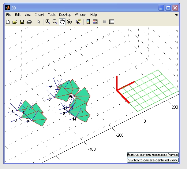
After you have made the camera calibration, you should have a result similar to the image bellow, after clicking on the Reproject on images option in the main menu. As you can see, if the calibration went without major problems, there should be one axis system ( resulting from the calibration ) attached to the chessboard in the same position as in the images above. By clicking on the Show extrinsic menu option, and then by clicking on the menu option inside the new window Switch to world centered view you should see the 3D view of the calibration. Again, here you can see the axis system attached to the chessboard resulting from the calibration.
|
|
|

The camera calibration results should be saved, because they will be needed in the future. In order to do that, click on the Save menu option to save the results. The resulting file will be used by our Toolbox, using the default filename provided by the Toolbox, 'Calib_Results.mat'.
:: The calibration procedure
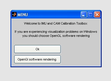
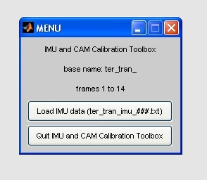
Now that we have all the information needed to make the calibration, we start the Toolbox, by writting in the Matlab command window the command imucam. The following welcome window will apear. In this window you can choose between the normal rendering or OpenGL rendering, usefull if you experiment some rendering problems during the Toolbox utilization.
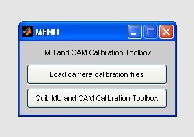
The next 2 windows will load the dataset: first the camera calibration file resulting from the camera calibration made before and the images, and then the files containing the inertial information.
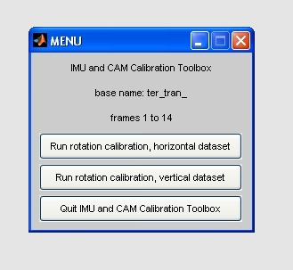
In this step its time to choose between vertical and horizontal calibration, depending on the dataset you have and your objectives: obtain the vertical vector if you have a horizontal dataset or obtain the vanishing pointing vector if you have a vertical dataset.
In this step you can start obtaining results from the Toolbox. If you check the Matlab command window you can see the calibration result, within a quaternion with the Euler angles:
IMU to CAM Rotation quaternion.
q =
-0.49713 <0.056827, 0.86444, 0.048723>
In the Menu we have now five options:
Show unit sphere and rotation for selected frame
Next frame (current frame = x)
Show rotation reprojection error
Save rotation quaternion to imu2cam.mat
Quit IMU and CAM Calibration Toolbox
Show unit sphere and rotation for selected frame
Inside this option the Toolbox shows the sphere reprojection of the current image and the corresponding vertical or vanishing pointing vectors depending on the calibration you make – horizontal or vertical. As you can see in the image bellow, a new figure apears, with the current image and respective reprojection inside the sphere. In this case, because it is a vertical dataset, the red vector is pointing towards the vanishing point in the image. On the Matlab command line you can see the resulting Euler angles for IMU to camera calculations and the resulting vanishing point vector.

Fig. 7 – unit sphere reprojection and vanishing point vector in red.

Fig 8 – Matlab global view including the command line.
Next frame (current frame = x)
By chosing this option you change from the current image to the next, to allow posterior reprojection into the unit sphere ( using the first option already mentioned before ).
Show rotation reprojection error
This option allows you to check the accuracy of the rotation angles obtained in the calibration. A good result should be under 1 pixel in the average error.
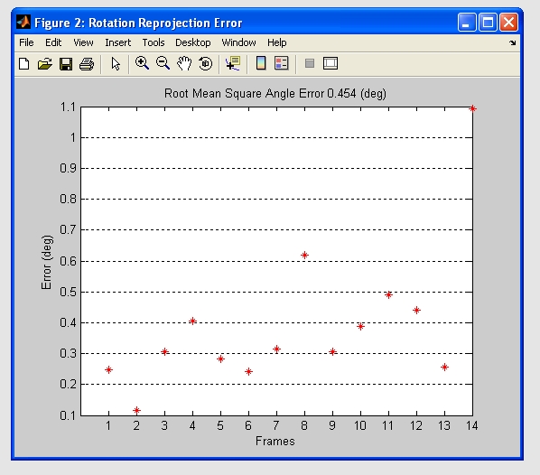
Fig. 9 – Rotation reprojection error for each image.
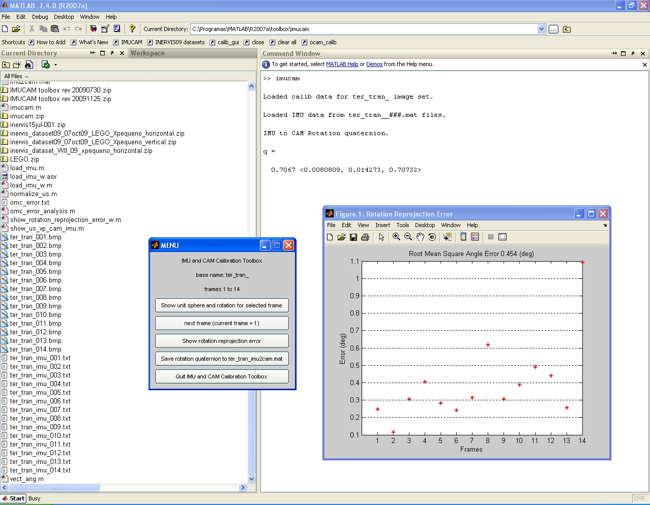
Fig. 10 – Matlab global view including the command line for the reprojection error.
Save rotation quaternion to imu2cam.mat
Allows you to save a file containing the Euler angles quaternion.
Quit IMU and CAM Calibration Toolbox
Exits the Toolbox.
You should now be able to use the Toolbox. If you have any questions please feel free to contact us.