Introduction
-
Motivation for Inertial and Vision Sensors Integration
- Inertial sensors attached to a camera can provide valuable
data about camera pose and movement. In biological vision systems,
inertial cues provided by the vestibular system, are fused with vision at an early processing stage.
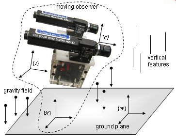
The 3D structured world is observed by the visual sensor, and its pose and motion parameters directly measured by the inertial sensors. These motion parameters can also be inferred from the image flow and known scene features. Combining the two sensing modalities simplifies the 3D reconstruction of the observed world. The inertial sensors also provide important cues about the observed scene structure, such as vertical and horizontal references.
The vestibular system plays an important role in human and animal vision. The vestibulo-ocular reflex is used for image stabilisation, and the sense of motion and posture is derived from inertial cues and visual flow. Vision processing also has “preferred” horizontal and vertical directions aligned with vestibular system
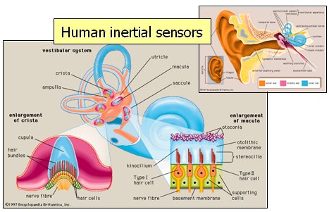
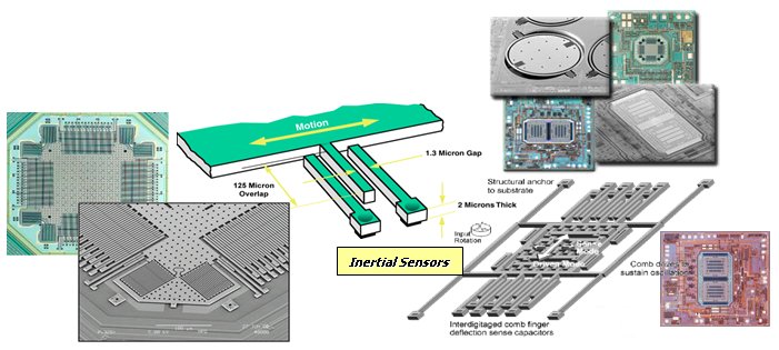
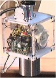
MEMs sensors and human vestibular system have similar performance. Single chip inertial sensors can be easily included in artificial vision systems, enabling the integration of artificial vision and inertial sensing for 3D reconstruction, visual navigation, augmented reality and related aplications.
-
Data from Inertial Sensors
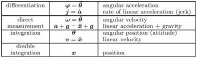
- Inertial sensors provide direct measurements of body
acceleation and angular velocity, from which other quantities can be
derived
-
Inertial Navigation Principles
At the most basic level, an inertial system simply performs a double integration of sensed acceleration over time to estimate position.
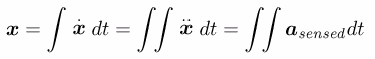
But since body rotations occur, this integration has to be done in the navigation frame of reference, as shown in this block diagram of a strapdown inertial navigation system.
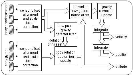
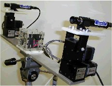
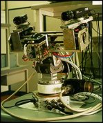
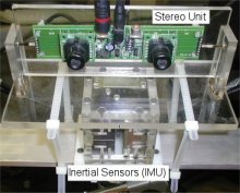
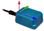
The inertial sensors, typically an orthogonal set of 3 accelerometers and 3 gyros, compose the IMU (Inertial Measurement Unit).
-
Data from Vision Sensors
-
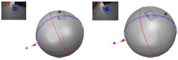
Projection onto Unit Sphere
Camera vision sensors provide images, with pixels corresponding to measurements of projective ray direction and colour or gray level intensity. This can be modeled with a projection onto a unit sphere as shown bellow
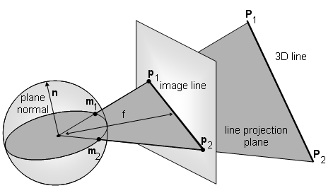
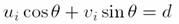
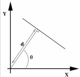
Image points are represented by projective ray direction m1, m2
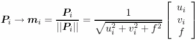
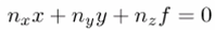
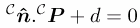
And image lines by the normal to the line projection plane n=m1 x m2
-
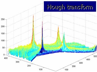
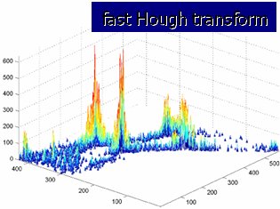
Vanishing Points and Vanishing Lines
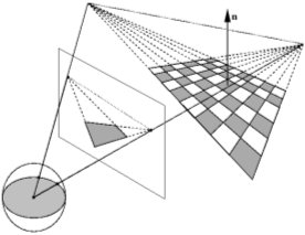
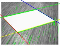
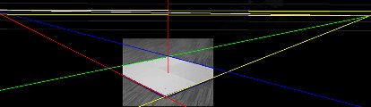
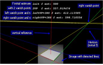
Under the camera projection, phenomena that only occurs at infinity will project to very finite locations in the image. The projection of parallel lines meet at their vanishing point. Under the unit sphere projection, the vanishing point given by line direction m=n1 x n2.
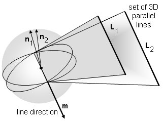
The set of vanising points of lines belonging to the same world plane define a common vanishing line
Vision and Inertial Sensing
-
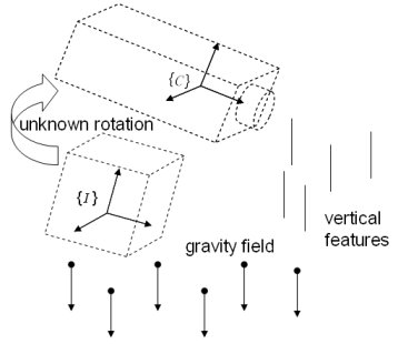
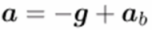
How does gravity show up in the camera?
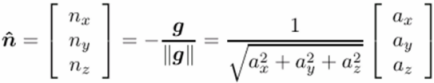
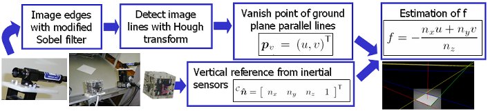
Inertial sensors provide an important external reference by sensing gravity.
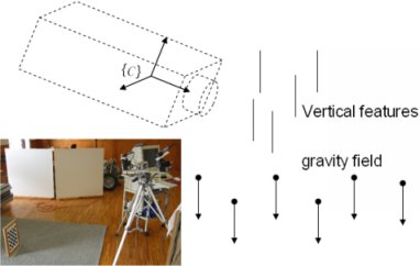
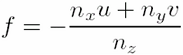
Gravity can also be observed by the camera as the vanishing point of vertical features.
-
How does linear and angular motion show up in the camera?
-
Optical flow and Spherical motion field
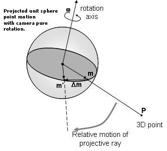
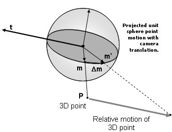
If the camera experiences both rotation ω and translation t the fixed world Pi given in the camera referential will have a motion vector given by
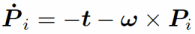
The motion field projected onto the unit sphere is given by
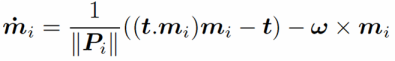
This equation describes the velocity vector for a given unit sphere point mi as a function of camera ego motion (t,ω) and point depth.
-
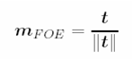
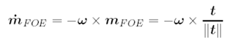
Image focus of expansion (FOE)
-
Image center of rotation (COR)
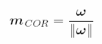
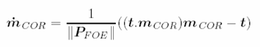
Both FOE and COR are known from inertial data alone (if system is calibrated).
-
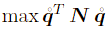
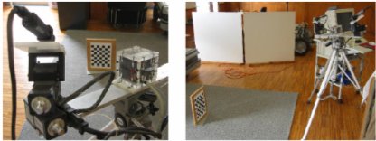
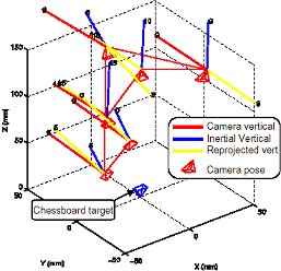
Frames of Reference
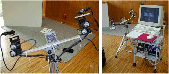
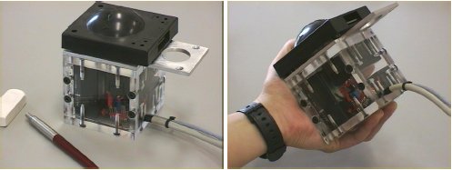
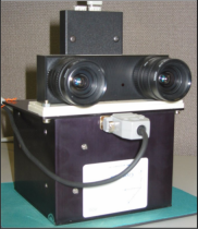
The camera and the inertail sensors in the IMU have different frames of reference.
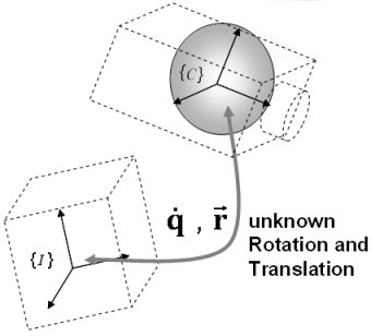
If the system uses a rigid mout, than the two are related by an unkown rotation and translation. In some cases this can be known, to some degree, from construction.
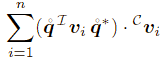
 where matrix
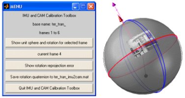
 ,
with
,
with 
 (avi 1.2MB)
 avi (2MB)
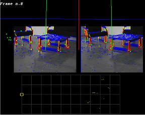 avi (3.2MB)
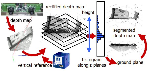
 mpeg movie
(3MB)
mpeg movie
(3MB)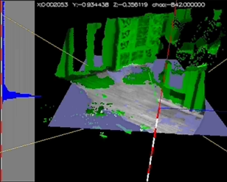 avi movie
(7.5MB)
avi movie
(7.5MB)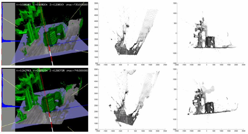