
:: Our work on Integration of Vision and Inertial Sensors
-
Introduction
-
Motivation for Inertial and Vision Sensors Integration
- Inertial sensors attached to a camera can provide valuable
data about camera pose and movement. In biological vision systems,
inertial cues provided by the vestibular system, are fused with vision at an early processing stage.
The 3D structured world is observed by the visual sensor, and its pose and motion parameters directly measured by the inertial sensors. These motion parameters can also be inferred from the image flow and known scene features. Combining the two sensing modalities simplifies the 3D reconstruction of the observed world. The inertial sensors also provide important cues about the observed scene structure, such as vertical and horizontal references.
The vestibular system plays an important role in human and animal vision. The vestibulo-ocular reflex is used for image stabilisation, and the sense of motion and posture is derived from inertial cues and visual flow. Vision processing also has preferred horizontal and vertical directions aligned with vestibular system
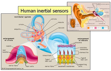
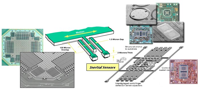
MEMs sensors and human vestibular system have similar performance. Single chip inertial sensors can be easily included in artificial vision systems, enabling the integration of artificial vision and inertial sensing for 3D reconstruction, visual navigation, augmented reality and related aplications.
-
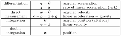
Data from Inertial Sensors
- Inertial sensors provide direct measurements of body
acceleation and angular velocity, from which other quantities can be
derived
-
Inertial Navigation Principles
At the most basic level, an inertial system simply performs a double integration of sensed acceleration over time to estimate position.
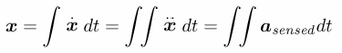
But since body rotations occur, this integration has to be done in the navigation frame of reference, as shown in this block diagram of a strapdown inertial navigation system.
The inertial sensors, typically an orthogonal set of 3 accelerometers and 3 gyros, compose the IMU (Inertial Measurement Unit).
-
Data from Vision Sensors
-
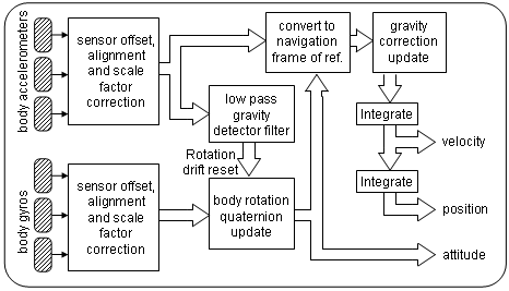
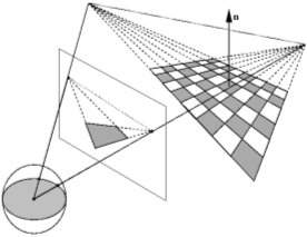
Projection onto Unit Sphere
Camera vision sensors provide images, with pixels corresponding to measurements of projective ray direction and colour or gray level intensity. This can be modeled with a projection onto a unit sphere as shown bellow
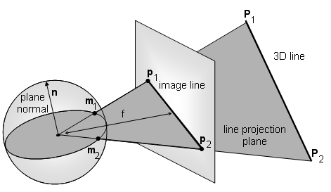
Image points are represented by projective ray direction m1, m2
And image lines by the normal to the line projection plane n=m1 x m2
-
Vanishing Points and Vanishing Lines
Under the camera projection, phenomena that only occurs at infinity will project to very finite locations in the image. The projection of parallel lines meet at their vanishing point. Under the unit sphere projection, the vanishing point given by line direction m=n1 x n2.
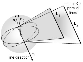
The set of vanising points of lines belonging to the same world plane define a common vanishing line
-
Vision and Inertial Sensing
-
How does gravity show up in the camera?
Inertial sensors provide an important external reference by sensing gravity.
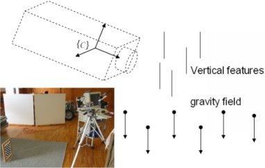
Gravity can also be observed by the camera as the vanishing point of vertical features.
-
How does linear and angular motion show up in the camera?
-
Optical flow and Spherical motion field
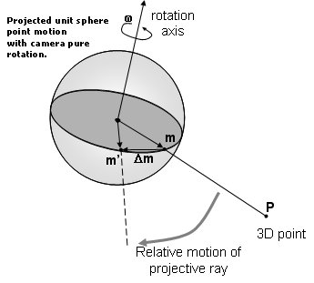
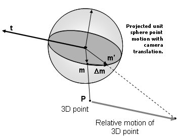
If the camera experiences both rotation ω and translation t the fixed world Pi given in the camera referential will have a motion vector given by
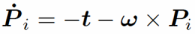
The motion field projected onto the unit sphere is given by
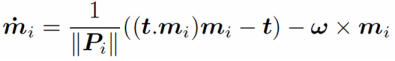
This equation describes the velocity vector for a given unit sphere point mi as a function of camera ego motion (t,ω) and point depth.
-
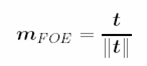
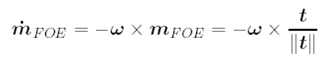
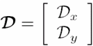
Image focus of expansion (FOE)
-
Image center of rotation (COR)
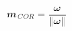
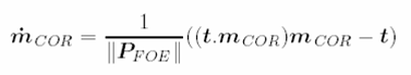
Both FOE and COR are known from inertial data alone (if system is calibrated).
-
Frames of Reference
The camera and the inertail sensors in the IMU have different frames of reference.
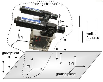
If the system uses a rigid mout, than the two are related by an unkown rotation and translation. In some cases this can be known, to some degree, from construction.
-
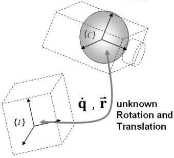
Calibrating Camera - IMU rotation and translation
Assuming a rigid mount between the camera and the IMU, we can assume a fixed rotation and a static boresight calibration method can be performed. If both sensors are used to measure the vertical direction, with a set of observations at different camera positions, the unknown rotation quaternion can be determined.
When the IMU sensed acceleration is equal in magnitude to gravity, the sensed direction is the vertical. For the camera, either using a specific calibration target, such as a chessboard placed vertically, or assuming the scene has enough predominant vertical edges, the vertical direction can be taken from the corresponding vanishing point. However camera calibration is need to obtain the correct 3D orientation of the vanishing points.
If n observations are made for distinct camera positions, recording the vertical reference provided by the inertial sensors and the vanishing point of scene vertical features, the absolute orientation can be determined using Horn's method. Since we are only observing a 3D direction in space, we can only determine the rotation between the two frames of reference.
Let Ivi be a measurement of the vertical by the inertial sensors, and Cvi the corresponding measurement made by the camera derived from some scene vanishing point. We want to determine the unit quaternion q that rotates inertial measurements in the inertial sensor frame of reference I to the camera frame of reference C. In the following equations, when multiplying vectors with quaternions, the corresponding imaginary quaternions are implied. We want to find the unit quaternion q that maximizes
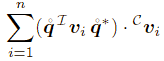
after some manipulation we want to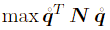 where matrix N can be
expressed using the sums for all i
of all 9 pairing products of the components of the two vectors Ivi
and Cvi. The
sums contain all the information that is required to find the solution.
where matrix N can be
expressed using the sums for all i
of all 9 pairing products of the components of the two vectors Ivi
and Cvi. The
sums contain all the information that is required to find the solution.
Since N is a symmetric matrix, the solution to this problem is the four-vector qmax corresponding to the largest eigenvalue of N, and a a closed form solution is obtained.
An inervis matlab toolbox was developed implementing this method.
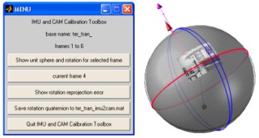
In a test sequence, the camera was moved through several poses with the vertical chessboard target in sight, and all IMU data and images logged. The camera calibration was performed with images sampled from the complete set recorded.
The figure below shows some of the reconstructed camera positions.
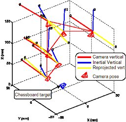
The estimated rotation has an angle 91.25° about an axis (0.89,−0.27,−0.3582), and is about the expected one,
given the mechanical mount, of a near right angle approximately about the x axis. Re-projecting the inertial sensor
data showed consistency of the method. The mean-square error in the re-projected verticals was 1.570◦.
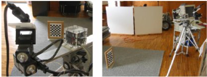
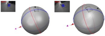
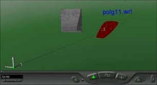
In another test, where 14 observations were made, the mean-square error in the re-projected verticals was 1.312°. The next table show this result and the error obtained using less observations,
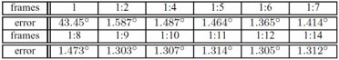
and below two of the frames used and corresponding unit shere model with the projected image, the vanishing point construction, the IMU measured vertical and its re-projection to the camera frame.
-
Results using Gravity as a Vertical Reference:
-
Vertical Reference
Accelerometers measure gravity vector g summed with body acceleration ab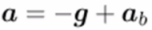
When system is motionless, gravity vector provides attitude reference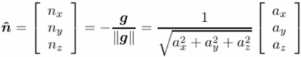
Gyros can be used to update the vertical reference when there is body acceleration.
-
Artificial Horizon
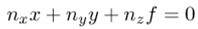
Having the vertical reference, the horizon line is know and given by
-
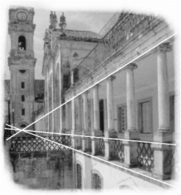
Camera Calibration with single vanishing point
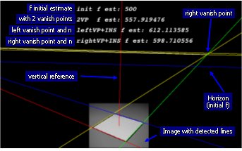
Using just one vanishing point, obtained from two parallel lines belonging to some levelled plane, and using the cameras attitude taken from the inertial sensors, the unknown scaling factor f in the cameras perspective projection can be estimated.
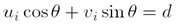
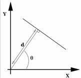
Given a single levelled plane vainishing point (x,y) in the image plane and the vertical reference n, the horizon line is given by
Focal distance f can be calibrated if camera and IMU are aligned or their rotation is known.
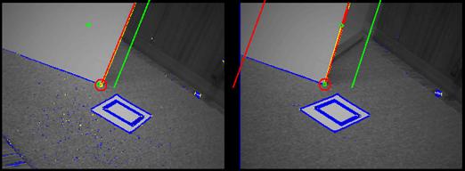
The proposed method is outlined below:
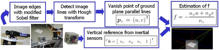
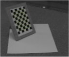
The camera is set to observe a simple scene of a levelled rectangle. The image gradient is computed using a modified Sobel filter that has a lower gradient direction angle error:
 ,
with
,
with 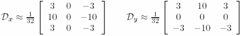
Image edges are obtained by thresholding the gradient magnitude and image line detection is done using the Hough transform
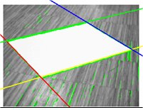
To speedup the computation a fast Hough transform is done using the gradient provided by the modified Sobel filter.
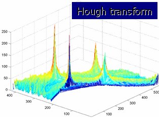
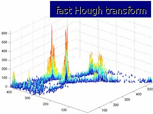
The highest peaks correspond to image lines. Vanishing points are given by line intersections:

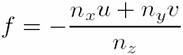
A vanishing point (u,v) of a set of parallel lines from a levelled plane belong to the horizon line, and hence f is given by
Shown bellow are some calibration results using this method.
A planar rectangular target was used and rotated through 19 positions, with 10 samples taken at each position
 (avi 1.2MB)
or animated gif (0.27MB)
(avi 1.2MB)
or animated gif (0.27MB)
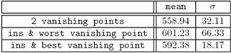
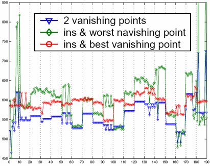
A lower error was achived using the vertical reference and nearer vanishing point, since the more unstable vanishing point is avoided.
In another test the Camera Calibration Toolbox for Matlab (based on Intel Open Source Computer Vision Library) was used as a standard for comparison. The matlab calibration was performed with 20 images of a chessboard target, obtaining f =617.57084 ± 10.35554 (shown by the blue line and shaded area in the chart below). For the Estimation of f with just one vanishing point and n, two target positions with a near vanishing point were used with 100 samples taken at each target position. The estimated f is shown in red in the chart below and has mean=613,02 and std=2,62.
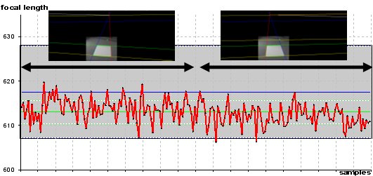
We can see that the proposed method provides a good estimate of f , within the uncertainty of the standard method.
The main sources of error are the vanishing point instability, evidenced by the stepwise results obtained in previous test, and the noise in the vertical reference provided by the low cost accelerometers. Nevertheless the method is feasible and provides a reasonable estimate for a completely uncalibrated camera. The advantage over using two vanishing points is that the best (i.e. more stable) vanishing point can be chosen. Another advantage is that in indoors environment the vanishing point point can sometimes be obtained from the scene without placing any specific calibration target, since. ground plane parallel lines can be easily detected.
-
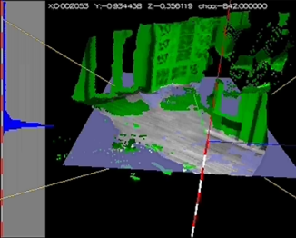
Ground Plane Segmentation
The ground plane is determied by the vertical reference n, up to unkown depth d
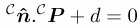
...
Sample of ground plane segmentation using Inertial Sensors and Active Vision
VRML Sample of ground plane segmentation using Inertial Sensors and Active Vision
 vrml
(VRML plug-in)
vrml
(VRML plug-in)
-
Vertical Feature Segmentation
Vertical reference n is the vanishing point of image line projections of world vertical features.
...
 avi (2MB)
or animated gif (0.67MB)
avi (2MB)
or animated gif (0.67MB)
 avi (3.2MB)
or animated gif (0.5MB)
avi (3.2MB)
or animated gif (0.5MB)
-
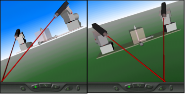
Stereo Depth Map Alignment
Another approach to inertial and vision sensor integration is to use standard vision techniques to compute depth maps, and than rotate and align them using the inertial reference. The advantage of reducing the search space explored above is lost, but current technology provides real-time depth maps with reasonable quality, and the inertial data fusion is still very useful at a later step to align and register the obtained maps.
Using the vertical reference, dense depth maps provided by a stereo vision system can be segmented to identify horizontal and vertical features. The aim is on having a simple algorithm suitable for a real-time implementation. Since we are able to map the points to an inertial reference frame, planar levelled patches will have the same depth z, and vertical features the same xy, allowing simple feature segmentation using histogram local peak detection. The diagram below summarizes the proposed depth map segmentation method.
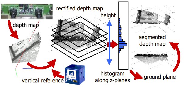
The depth map points are mapped to the world frame of reference. In order to detect the ground plane, a histogram is performed for the different heights. The histogram's lower local peak, zgnd, is used as the reference height for the ground plane.
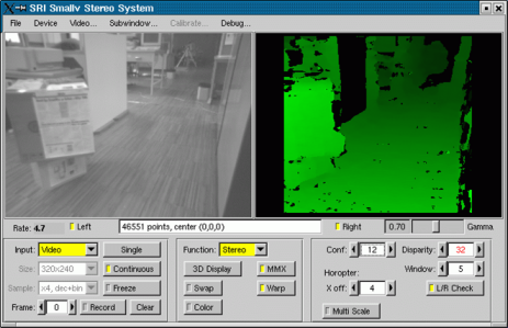
We are using the Small Vision System (SVS) from SRI to obtain real-time depth maps since they provide an efficient implementation of area correlation stereo. The linux version is shown below, computing a depth map for the oberved scene.
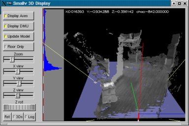
Adding to the static view provided by the standard SVS, we programed a 3D dynamic view, incorporating a rotation to the inertial reference and ground plane detection. This and other results of ground plane detection and depth map rectification are shown below.
 mpeg movie
(3MB)
mpeg movie
(3MB)
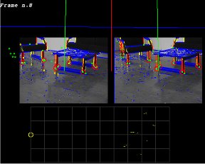
Another movie with points above the floor shown in green:
 avi movie
(7.5MB) or
avi movie
(7.5MB) or
Set of resuts with top and side view of alinged 3D point cloud:
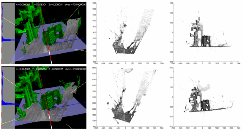
Dynamic inertial data provides aproximation for 2D translation and rotation registration of depth map points.
-
Results using Velocity and Acceleration
-
Experimental setups used
-
First Inertial System Prototype
- First Inertial System Prototype for use with a mobile robot
-
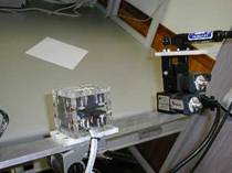
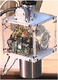
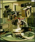
InerCube
- After the initial tests with the inertial sensors, we chose
to build our own inertial measurement unit prototype. We were able to
tailor the system to our specific needs, and gain a better insight into
the technology, working towards a low-cost inertial and vision system
for robotic applications, within the available budget. The sensors used
in the prototype system include a three-axial accelerometer, three
gyroscopes and a dual-axis inclinometer. A temperature sensor is also
included to enable implementation of temperature error compensation.
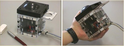
The three-axial accelerometer chosen for the system, while minimising eventual alignment problems, did not add much to the equivalent cost of three separate single-axis sensors. The device used was Summit Instruments 34103A three-axial capacitive accelerometer. In order to keep track of rotation on the x-, y- and z-axis, three gyroscopes were used. The piezoelectric vibrating prism gyroscope Gyrostar ENV-011D built by Murata was chosen. Initially tilt about the x and y-axis was measured with a dual axis AccuStar electronic inclinometer, built by Lucas Sensing Systems (now schaevitz). The inertial sensors were mounted inside an acrylic cube, enabling the correct alignment of the gyros, inclinometer (mounted on the outside) and accelerometer, as can be seen above. This inertial system can measure angular velocity with 0.1 deg.s−1 resolution, and linear acceleration with 0.005 g resolution.
-
InerCube on robotic active vision head
-
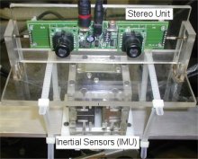
InerCube and Stereo Cameras with Pan&Tilt units
-
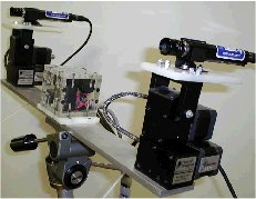
VRML demo of Active Vision System with two Pan&Tilt units. (VRML plug-in)
-
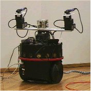
InerCube and SVS analog stereo
-
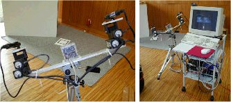
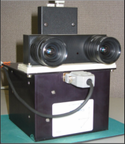
CrossBow DMU and Mega-D SVS firewire stereo
-
-
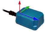
Xsens MT9-B IMU and firewire digital camera
